Download and Install
Download and install the following software:
- QGIS 1.7.3
- Postgres/PostGIS 9.1.2-1 (x86-32)
- TileMill 0.9
QGIS and TileMill are straight forward. Postgres installs first (take note of your username and password) then launches the Application Stack Builder for installing PostGIS. Check off PostGIS and the ODBC connector is also handy when connecting to Microsoft formats.
 Download data

We will use data from several sources to for our analysis and maps.
- OSM data for a base map
- Census TIGER\Line county shape files
- Census TIGER\Line zipcode shape files
- Texas Education Agency school shape files
- Texas Education Agency school district shape files
- Texas Education Agency school campus dropout rates CSV file
- Texas Education Agency school district dropout rates CSV file
Download the shape files and unzip them into a single directory. Note that the TEA (Texas Education Agency) site assigns the same name to both the campus and district dropout rate csv files, so use the 'Save as' option to give the files unique names when downloading the files. Also of importance are the metadata describing the TEA files.
Loading spatial data into PostGIS
I'll start by saying PostGIS isn't necessary for spatial analysis. Shape files, geoson,spatialite, etc are all perfectly acceptable data formats that can be consumed by QGIS and/or TileMill. The main advantage of using PostGIS in this context is data management with the added bonus of being able to performing spatial operations if you are willing to learn SQL. We'll touch on using SQL in subsequent articles but as always there is more than one way to do any task. For those not quite ready to jump into learning SQL, QGIS can act as front end for PostGIS.
Buckets
Postgres is a relational database and there are a number of best practices associated with building and maintaining transactional databases. We're going to chuck all of that aside, because like the honey badger, spatial data doesn't care about 3rd normal form or referential integrity. We're going to treat databases as big buckets of gooey geo goodness.
First we're going to create a database using PGAdmin III, which is a graphical frontend for Postgres included in the install.


Now that we have a connection to the data base, click 'Connect' to establish the connection. We will use the default SRID, since all the shape files are in the same projection. Click 'Add' and select the OSM, Census and the reprojected TEA shape files. Click 'OK' to load them into PostGIS. This make take a bit of time, especially for the larger files such as the OSM highways file.
 You can check that the data was imported using PGAdmin III. Press 'F5' to refresh the view and click on the 'texas' database to open the tree view, then click on 'Tables' to view them.

Data prep using command line tools
Advocacy for open data has made more data available in the web; but often the data is in an 'as-is' state that requires additional refinements to make it usable. The TEA dropout rate data is no different and it is important to look at the data to determine what the individual columns mean and if they are in a format that is suitable for analysis.
Things to look out for are tocheck that data type is consistent and the data can be accurately and consistently represented as continuous or categorical values. CSV files come in many flavors and when importing the data into any database requires a degree of data sleuthing to ensure the data is imported correctly. There are many tools for examining and modifying data that range from text editors and spreadsheets. My preferred method is to use unix utilities such as sed, awk, and tr because they don't have file size or row limits found in text editors or spreadsheets.
If you have a preferred method feel free to skip ahead to the loading CSV into Postgres section. This part will describe how to use unix utilities to correct the CSV files and also write SQL scripts to create tables to hold the TEA dropout rate data. One of many pleasant surprises of QGIS for Windows is that it includes MSYS which is a collection of gnu utilities such as sed, awk, tr, and vi. Unlike Cygwin, it is not a full environment that includes the gcc compiler. It has a smaller foot print and provides just what is needed for manipulating data.
If we look at the header and first line of data in the campus dropout rate CSV file, we see that they each entry is quoted and comma delimited. That's OK for the header, but quoted data means that it will be imported as text into a database. Furthermore, if we look through out the data set, we see that many of the fields contain a mixture of numeric and text data. If you read through the site metadata, it says the some fields are purposely obfuscated to preserve privacy. That's the reason why some of the data contains a less than sign in front of the value. Here are a couple of examples on how to use head and tail to look at various parts of a file.
One of the problems with the files is that null or empty values are represented by ".", this is unacceptable. We'll fix this by removing the values using sed, which is a utility that edit a file as stream instead of opening the entire file at one time. You can find and replace values using substitution. The general form of substitution in sed takes the form of 's/text to replace/new text/g'. The 's' means substitution and the 'g' means global or the perform this on the entire file. In the example below, we will need to escape the quote and period with a backslash because they are special characters. The version of sed in MSYS does not support in place editing, so we will redirect the output using '>' to another file. Finally, we remove the column headers in the file by copying it to a tmp file, then using sed to remove the first line. The file 'campus_dropout_clean.csv' is now ready for importing into Postgres. Repeat the same process for the district file.
However, before we can import the data, we will need to define and create the table structure in Postgres using SQL. The CREATE TABLE statement is straightforward and can be done by typing it into psql or the PGAdmin SQL console. I'll be the first to admit that I'm a terrible typist and very prone to error. To overcome my lack of typing skills I use sed to create the SQL.
I start with the header line of the CSV file because it contains all the column names. I use head to grab the first line and save it to 'campus_header' file. This file has all the column names in a single line, so I use sed to to add a newline and write the output to 'campus_dropout_raw.sql' file. Note that I use an actual carriage return instead of the newline ('\n') because of a limitation in sed. Use 'cat' to see the new file.
To finish up the SQL we'll add the CREATE TABLE statement and the closing parentheses using sed. We want to only operate on the first line of the file so we user '1s' to perform the substitution. Note that the output is redirected to a temporary file because this version of sed lacks in place editing. We take the temp file and add the varchar type definition and closing parentheses using sed again. Note that we want to only operate on the last line of the file so we use '$s'. The output is redirected to the 'campus_dropout_raw.sql' file.
Now we have a SQL file to create the table holding the raw TEA campus dropout rates. One of the problems of the file is that all the data is mixed between numeric and text types especially for the fields used to calculate the rate. Fortunately, the dropout rate fields contain the calculated rate as numeric values. We can create a table with the dropout ratio defined as a numeric value instead of a character string. Later on, we will use the raw data to populate the actual dropout rate table.
In the previous example we wanted to get all the column names, but in this example we want to get just the column names with the different dropout rates. We use tr to add carriage returns after the comma then send it to sed to extract the fields of interest. Luckily, the dropput rates occur in a regular pattern so we use '2~3p' to specify that starting on the second line extract every third line in the file. We then send the ouput to a file called campus_dropout_rate.sql.
If we look at the output file using cat, we can see it extracted the desired lines plus a few extra at the end. To get a clean file of only the dropout rate fields we extract the first 21 lines and redirect it to a 'tmp' file. To get the count of the lines we want, use wc to get the total number of lines and subtract the lines you don't want. Add the numeric type definitions using sed and redirect the output to the 'first' file.
The remaining nine fields in the campus_header file are useful fields that contain the campus identifier as well as other important information such as school name. We want those fields so we extract them using tr and tail and write the results to a 'tmp' file. As in the previous example, add the varchar type definition using sed and write the output to the 'last' file. We glue the 'first' and 'last' file using the cat command and redirect the output to the campus_dropout_rate.sql file. Finally, we finish by adding the CREATE TABLE statement and closing parentheses was we did in the previous example.
In this section, we used command line utilities to clean up files and create SQL scripts to create tables in Postgres. Repeat the process for the district dropout rate data. When we have completed the cleaning and making SQL scripts for the district data, we'll be ready to import the data into Postgres.
Importing CSV files into Postgres
In this section we will use PGAdmin and the SQL editor to load the data. Open PGAdmin III, select the 'texas' database, and click on the 'SQL' button to launch the SQL editor.
 In the SQL query window, click on the 'File'>'Open' to open the campus_dropout_raw.sql file. Load the file, then click on Click on 'Query'>'Execute' to run the script.
 Repeat the same process for the campus_dropout_rate.sql, district_dropout_raw.sql, district_dropout_rate.sql files. You should have four new tables listed when you are finished.
The final step is to import the raw data and insert the cleaned data in to the campus and district rate tables. Postgres provides the COPY command to import text files into tables. You can use the SQL window to write and execute SQL. Clear the the window by clicking on 'Edit'>'Clear window' and type the following and substituting the appropriate path.
 The next step is to populate the campus_dropout_rate table from the table containing the raw data. To do this, we use and INSERT statement to copy the data and convert the data to a numeric type. Using the same techniques in the previous example, I created this script.
Copy and past the script into the SQL window and run the script.
 Repeat the same process for the district data. That's it for loading the tabular TEA data on campus and district dropout rates. Later on, we will join the tables to the school and district PostGIS layers for analysis.
Summary
We've done a lot - installed software, created a database, reprojected and loaded shape files in PostGIS using QGIS, used command line tools to clean up CSV files and create SQL scripts, and finally created tables and loaded data in Postgres. While some of this may seem complicated (especially the command line portion), this is the type of work flow I would use if someone asked me to make a map of data pulled from the Internet. It's the kind of workflow that I used as a GIS analyst in a previous life to overcome the shortcomings of spreadsheets and text editors as data cleaning tools. Overall, I'm impressed that I can do all of this in Windows with just QGIS and Postgres.
The following article will cover spatial analysis in QGIS and Postgres. We'll look at QGIS plug-ins and exercise the spatial functions in PostGIS.
Buckets
Postgres is a relational database and there are a number of best practices associated with building and maintaining transactional databases. We're going to chuck all of that aside, because like the honey badger, spatial data doesn't care about 3rd normal form or referential integrity. We're going to treat databases as big buckets of gooey geo goodness.
First we're going to create a database using PGAdmin III, which is a graphical frontend for Postgres included in the install.
Your Postgres instance should be already connected but in case it isn't, please see this page. Add a new database by right clicking on 'Databases'>'New Database'

Name the new database 'texas'

Click on the 'Definition' tab, and select 'template_postgis' as the Template and click 'OK'. Template_postgis is a predefined database that contains the Postgis tables and spatial functions. Congratulations, you've made a bucket!

Reprojecting data in QGIS
Previously we downloaded a number of shape files from the Census, TEA and Cloudmade's OpenStreet Map extract of Texas. It's always a good idea to check the .prj or metadata files associated with the shape file. The OSM and Census files are both in WGS84, but the TEA files are in the Texas Centric Mapping System projection. For the purposes of this project, we'll use QGIS to reproject the TEA files to WGS84. Then load the shape files using SPIT in QGIS.
First add the TEA shape files. Click on Layer>Add Vector Layer

Browse to the directory the TEA files are in and select them. Click OK to complete.

Select 'Schools2010' and right click and select 'Save as...'

Browse to the directory to save the file and name it 'tea_school_campus'

Next we'll set the output CRS (projection) to WGS84. Click 'Browse' on the CRS field and select WGS84 under the 'Geographic Coordinate Systems' list or use the 'Search' box to find it. Click 'Ok' with WGS84 selected. Then click 'OK' to reproject and save the file.

Repeat the same process for the Districts_10_11 shape file.
From QGIS to PostGIS
We'll use SPIT (Shapefile to PostGIS Import Tool) to import the shape files into PostGIS. Click 'Database'>'Spit'>'Import Shapefiles to PostGIS'

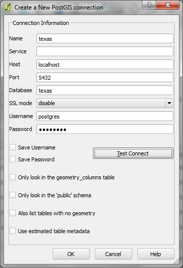
In the Spit window, create a connection to PostGIS by clicking on 'New'. Fill out the 'Name' (texas), 'Host' (localhost)', 'Database' (texas), 'Username' (postgres), 'Password' (your password). Save your user name and password if desired. Click on 'Test Connect' to test the connection; if successful, click 'OK' to save the connection.


Data prep using command line tools
Advocacy for open data has made more data available in the web; but often the data is in an 'as-is' state that requires additional refinements to make it usable. The TEA dropout rate data is no different and it is important to look at the data to determine what the individual columns mean and if they are in a format that is suitable for analysis.
Things to look out for are tocheck that data type is consistent and the data can be accurately and consistently represented as continuous or categorical values. CSV files come in many flavors and when importing the data into any database requires a degree of data sleuthing to ensure the data is imported correctly. There are many tools for examining and modifying data that range from text editors and spreadsheets. My preferred method is to use unix utilities such as sed, awk, and tr because they don't have file size or row limits found in text editors or spreadsheets.
If you have a preferred method feel free to skip ahead to the loading CSV into Postgres section. This part will describe how to use unix utilities to correct the CSV files and also write SQL scripts to create tables to hold the TEA dropout rate data. One of many pleasant surprises of QGIS for Windows is that it includes MSYS which is a collection of gnu utilities such as sed, awk, tr, and vi. Unlike Cygwin, it is not a full environment that includes the gcc compiler. It has a smaller foot print and provides just what is needed for manipulating data.
If we look at the header and first line of data in the campus dropout rate CSV file, we see that they each entry is quoted and comma delimited. That's OK for the header, but quoted data means that it will be imported as text into a database. Furthermore, if we look through out the data set, we see that many of the fields contain a mixture of numeric and text data. If you read through the site metadata, it says the some fields are purposely obfuscated to preserve privacy. That's the reason why some of the data contains a less than sign in front of the value. Here are a couple of examples on how to use head and tail to look at various parts of a file.
One of the problems with the files is that null or empty values are represented by ".", this is unacceptable. We'll fix this by removing the values using sed, which is a utility that edit a file as stream instead of opening the entire file at one time. You can find and replace values using substitution. The general form of substitution in sed takes the form of 's/text to replace/new text/g'. The 's' means substitution and the 'g' means global or the perform this on the entire file. In the example below, we will need to escape the quote and period with a backslash because they are special characters. The version of sed in MSYS does not support in place editing, so we will redirect the output using '>' to another file. Finally, we remove the column headers in the file by copying it to a tmp file, then using sed to remove the first line. The file 'campus_dropout_clean.csv' is now ready for importing into Postgres. Repeat the same process for the district file.
However, before we can import the data, we will need to define and create the table structure in Postgres using SQL. The CREATE TABLE statement is straightforward and can be done by typing it into psql or the PGAdmin SQL console. I'll be the first to admit that I'm a terrible typist and very prone to error. To overcome my lack of typing skills I use sed to create the SQL.
I start with the header line of the CSV file because it contains all the column names. I use head to grab the first line and save it to 'campus_header' file. This file has all the column names in a single line, so I use sed to to add a newline and write the output to 'campus_dropout_raw.sql' file. Note that I use an actual carriage return instead of the newline ('\n') because of a limitation in sed. Use 'cat' to see the new file.
To finish up the SQL we'll add the CREATE TABLE statement and the closing parentheses using sed. We want to only operate on the first line of the file so we user '1s' to perform the substitution. Note that the output is redirected to a temporary file because this version of sed lacks in place editing. We take the temp file and add the varchar type definition and closing parentheses using sed again. Note that we want to only operate on the last line of the file so we use '$s'. The output is redirected to the 'campus_dropout_raw.sql' file.
Now we have a SQL file to create the table holding the raw TEA campus dropout rates. One of the problems of the file is that all the data is mixed between numeric and text types especially for the fields used to calculate the rate. Fortunately, the dropout rate fields contain the calculated rate as numeric values. We can create a table with the dropout ratio defined as a numeric value instead of a character string. Later on, we will use the raw data to populate the actual dropout rate table.
In the previous example we wanted to get all the column names, but in this example we want to get just the column names with the different dropout rates. We use tr to add carriage returns after the comma then send it to sed to extract the fields of interest. Luckily, the dropput rates occur in a regular pattern so we use '2~3p' to specify that starting on the second line extract every third line in the file. We then send the ouput to a file called campus_dropout_rate.sql.
If we look at the output file using cat, we can see it extracted the desired lines plus a few extra at the end. To get a clean file of only the dropout rate fields we extract the first 21 lines and redirect it to a 'tmp' file. To get the count of the lines we want, use wc to get the total number of lines and subtract the lines you don't want. Add the numeric type definitions using sed and redirect the output to the 'first' file.
The remaining nine fields in the campus_header file are useful fields that contain the campus identifier as well as other important information such as school name. We want those fields so we extract them using tr and tail and write the results to a 'tmp' file. As in the previous example, add the varchar type definition using sed and write the output to the 'last' file. We glue the 'first' and 'last' file using the cat command and redirect the output to the campus_dropout_rate.sql file. Finally, we finish by adding the CREATE TABLE statement and closing parentheses was we did in the previous example.
In this section, we used command line utilities to clean up files and create SQL scripts to create tables in Postgres. Repeat the process for the district dropout rate data. When we have completed the cleaning and making SQL scripts for the district data, we'll be ready to import the data into Postgres.
Importing CSV files into Postgres
In this section we will use PGAdmin and the SQL editor to load the data. Open PGAdmin III, select the 'texas' database, and click on the 'SQL' button to launch the SQL editor.


The final step is to import the raw data and insert the cleaned data in to the campus and district rate tables. Postgres provides the COPY command to import text files into tables. You can use the SQL window to write and execute SQL. Clear the the window by clicking on 'Edit'>'Clear window' and type the following and substituting the appropriate path.

Copy and past the script into the SQL window and run the script.

Summary
We've done a lot - installed software, created a database, reprojected and loaded shape files in PostGIS using QGIS, used command line tools to clean up CSV files and create SQL scripts, and finally created tables and loaded data in Postgres. While some of this may seem complicated (especially the command line portion), this is the type of work flow I would use if someone asked me to make a map of data pulled from the Internet. It's the kind of workflow that I used as a GIS analyst in a previous life to overcome the shortcomings of spreadsheets and text editors as data cleaning tools. Overall, I'm impressed that I can do all of this in Windows with just QGIS and Postgres.
The following article will cover spatial analysis in QGIS and Postgres. We'll look at QGIS plug-ins and exercise the spatial functions in PostGIS.

No comments:
Post a Comment